Inflation: A Monetary Phenomenon

If you have ever been curious about how money works, then like me, you would have eventually crossed paths with inflation. A buzzword thrown around by politicians and the mainstream media, yet no one seems to really understand what it is nor why it exists. In the rare case someone does try to address the origin of inflation it is often a mere exercise in 'passing the buck', quite literally too. Whilst these so called "explanations" do provide some level of truth - it would be a stretch to call them origin stories for why inflation comes about in an economy. Follow along to uncover, what I believe to be, a very sound argument for the origin of inflation and what we can do to manage it.

The Plan

Without becoming just another opinion piece tumbling off the conveyor belt and being shipped off to fill the shelves of our politically charged slop shop we call the news industry - I will instead present my entire argument around evidence and the occasional opinions to support and interpret the results. I will be focusing on finding statistically significant evidence to back my claims - performing my own investigation into the matter from first principles.

The primary strategy for this investigation will be to employ what is called a multi-linear regression analysis. This will help us quantify correlations and relationships between variables of interest. It is important to note that this type of investigation alone does not in any way infer or prove causation, and this is something important we will touch on later.

The Idea

This is the explanation I not only subscribe to, but continue to turn to, when faced with answering the ultimate question of what really is inflation? It is too much money chasing too few goods.

If we hope to support this ideology with empirical evidence, then what we need to do is show that changes in the money supply are met with proportionate changes in inflation - holding all else equal.

\[ M\cdot V=P\cdot Y \]

This is the equation of exchange that shows how money supply \(M\), money velocity \(V\), price level \(P\), and output \(Y\) all relate to one another. We will take this as an assumption to build our case from here on out. But, before doing so, we will convert this to a growth rate equivalent form:

\[ \pi = \mu -g + v \]

It is hypothesized by monetarists that, in the long run, the velocity of money becomes stable/constant which means \( v\approx 0 \) leading \( \pi = \mu -g \). Of course, in the short run as observed in a real-life sample of data like that which we are investigating today – the velocity of money is not stable. It is important to understand though that should we one day have access to thousands or hundreds of thousands of data points – the model would likely converge to a more faithful representation in line with the hypothesized result. The model we will be constructing will therefore be as follows:

\[ \pi = \beta_0 + \beta_1 (\mu - g) + \epsilon \]

Where,

• \(\pi\) is inflation.
• \(\beta_0\) is the intercept whose economic meaning is somewhat left up to our own interpretation, I’ll touch more on this later.
• \(\beta_1\) is the coefficient of money supply growth (less the impact of real GDP growth).
• \(\mu\) is the money supply growth rate.
• \(g\) is the real GDP growth rate.
• \(\epsilon\) is the error term.

We can source the data we need to investigate this problem from various places – my preferred database is FRED. We’ll want the money supply growth rate, the real GDP growth rate and of course, inflation. I would recommend we sample annually on all 3 data types for consistency as some statistics are published monthly or quarterly etc.

Using a linear regression, we can estimate what \(\beta_0\), \(\beta_1\) are and determine if these values are statistically significant from zero. We therefore expect \( \beta_1 \) to be close to unity in long‑run averages, recognising that institutional and measurement effects may introduce deviations. Now, it is important to understand that formally there is a set of criteria that needs to be adhered to before drawing conclusions from these regressions – for the most part we meet them though we are limited by the amount of data points available to us. So, as it stands, it is so far unknown whether the residuals of the following regression adhere to a normal distribution – if they don’t then our estimators derived in the following sections will not mean much. Given the limited number of long‑run observations, formal diagnostic testing is constrained. Results should therefore be interpreted as descriptive rather than definitive.

A word on the intercept \( \beta_0 \) and its interpretation, if it is shown that the intercept is statistically significant i.e. non-zero, then we are left with a static metric that contributes to the explanatory power of the model. That is to say, when the independent variable (money supply growth less real GDP growth) is zero, the dependent variable – inflation is equal to \( \beta_0 \) on average. This means, at least over the sample period, there is some non-zero rate of inflation observed in the absence of changes in the supply of money. I will address this concern in later sections should it present itself.

10YR Trailing Averages

We will start our analysis with 10 year trailing averages of the data points, to assess the validity of any proposed relationship between money supply changes and inflation we need to be working in the order of many years or even many decades – this is because the short run economics will mask the long run trends which we are interested in.

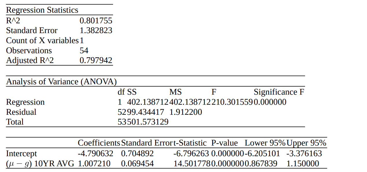
This model shows that money supply growth explains about 80% of the variance in inflation – the entire model is statistically significant with F-statistic ~ 0. Both the intercept and the coefficient of the independent variable are individually significant as shown with their respective p-values ~ 0. The coefficient of (M – G), \( \beta_1 = 1 \), is in line with our proposed hypothesis in the earlier discussions and in fact we can be 95% confident the value lies in the range [0.87, 1.15]. The intercept, however, is shown to be non-zero with \( \beta_0 = -4.79 \), the economic meaning of this variable is discussed in the later sections.

20YR Trailing Averages

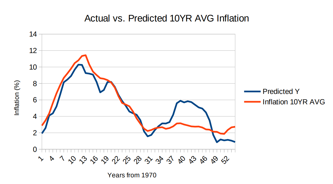
As shown from the previous regression we had a convincing trend until about 2006 – 2018 where predicted inflation far exceeded actual inflation. It is expected to see such short run variations in the trends; the economy is full of noise and forces acting in all directions in the short run – what matters to us is the long run relationship. 10 years was a good place to start but “long run” is frankly undefined and so we might as well double the time horizon to see what effect this has.

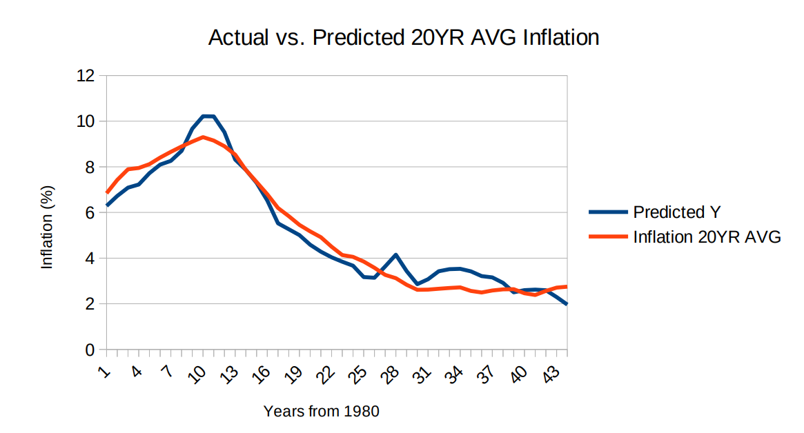
We can see that the 20-year averaging has increased the overall performance of the model. Now 95% of the variance observed in the inflation rate is explained by changes in the money supply – whilst this appears impressive, the usefulness of the estimators of this regression is impacted from potential over fitting. The coefficient of money supply growth has increased from about 1 to 1.4 which raises red flags given we know from theory to expect something close to 1. This also has implications for the interpretation of the intercept as discussed in the following section.

The Intercept

Let us unpack the meaning of the intercept in these two regressions, it is both statistically significant and non-zero in each case and so we should do our best to address why this may be. In our 10 year trailing averages regression we saw that \( \beta_1 \approx 1 \) which is exactly what we were hoping to see from the hypothesized results, this is important because if this coefficient agrees with the Quantity Theory of Money, then it allows us to offer an explanation for what the intercept is. The 10-year regression gave rise to \( \beta_0 = -4.79% \), so building out our model we have:

\[ \pi = (\mu - g) - 4.79% \]

Comparing this to the formal QTM relation:

\[ \pi = (\mu - g) + v \]

We see that the intercept must be an estimate for 10 year trailing average money velocity growth. To really drive this home, we can compare our estimate for average velocity growth to that derived directly from the data. We have \( \pi, \mu, g \) which means we can solve for \( v = \pi - \mu + g \). We can find each period’s velocity and then average across the entire sample period like so:

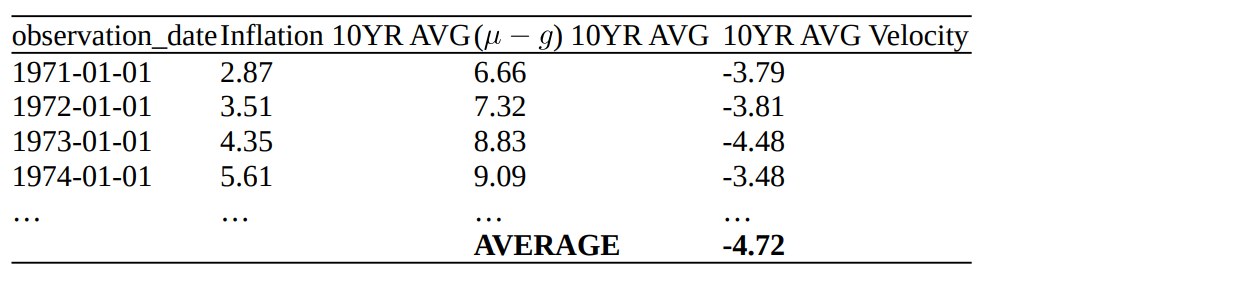
Here we see that averaging the 10YR trailing averages of money velocity gives a value of -4.72% which is very close to our regression estimate of -4.79% – demonstrating that our intercept of the regression is indeed an estimate of the average observed change in money velocity over the sample period.

Here is the implied velocity of money trend in Australia:

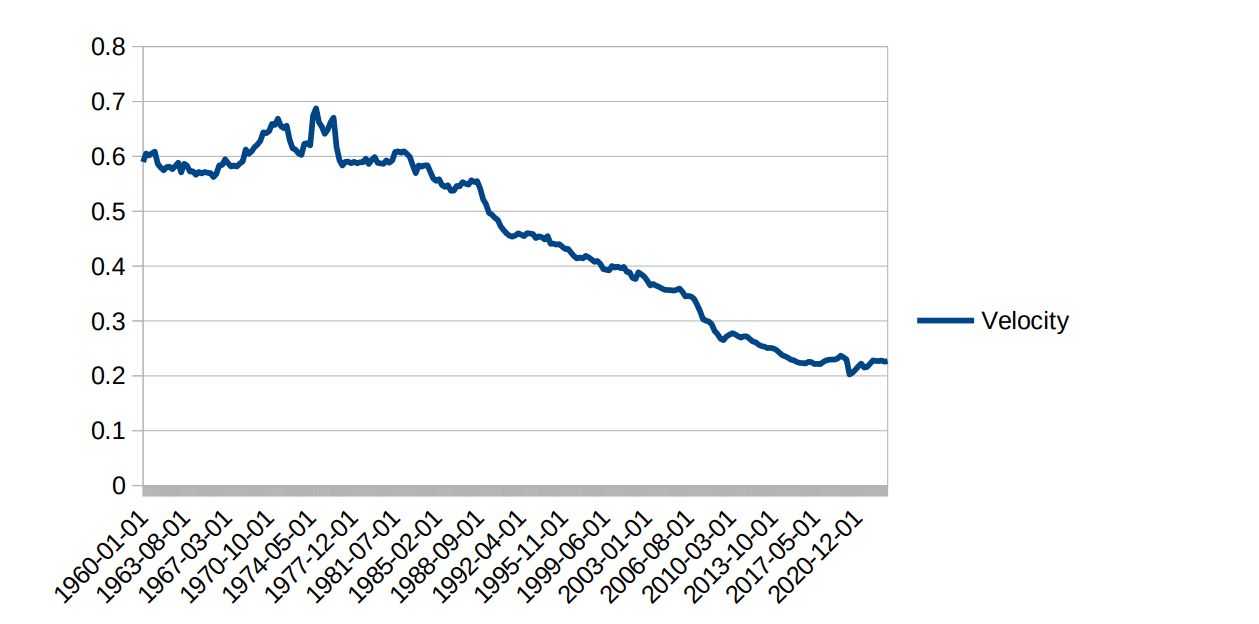
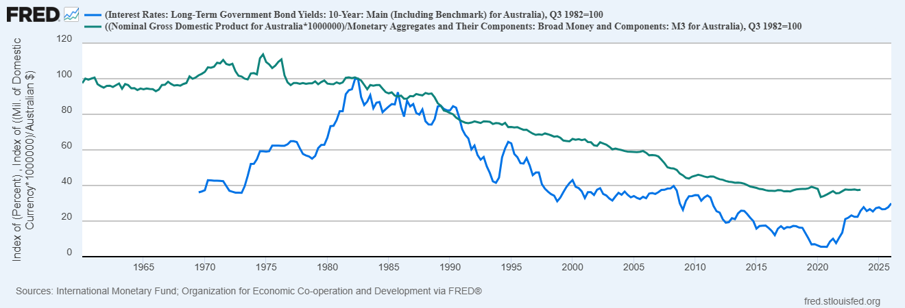
You can see from the above chart that money velocity has been steadily declining over time in what appears to be a relatively constant growth rate on average. The intercept of our regression captured this effect nicely by coincidence - had this velocity trend not been so uniform and steady - we would have needed to include some other variable to account for velocity movements in the model. This would usually be done with some sort of proxy such as the opportunity cost of holding money observed through policy interest rates or government bond yields, and in a more contemporary sense, some specific cryptocurrency statistics can offer similar insights too. A comparison between bond yields and implied money velocity is shown below to illustrate this point:

When looking at our 20-year trailing average regression – we can attempt to apply the same logic to reason with the intercept term. This regression produces \(\beta\approx 1.40\) with a 95% confidence interval of [1.29, 1.50] which is well above 1. This is not the result we were looking for and differs from our 10 year trailing averages regression. In this case the intercept cannot be directly associated with money velocity as before, and this is likely due to the fact discussed above - we are imposing an assumption that money velocity is stable when in reality it may not be. Without modelling velocity dynamics the model is biasing the estimators under such assumptions.

It is also worth noting that dropping from 54 observations to 44 via the extension of trailing average durations (10 to 20 years) means we are forced to fit against a smaller sample size which includes short run variations and noise in the economy – given the very limited data points available, the 10YR trailing averages model offers more meaningful insights which agree with, and can be explained by, the underlying Quantity Theory of Money without yet needing to explicitly model velocity dynamics.

This has demonstrated to a high degree of certainty that inflation is correlated to long-run movements in the money supply. Being able to predict long-run inflation solely on the money supply growth rate (excluding the relative effects of productivity in the economy by subtracting real GDP growth) is a testament to Milton Friedman and the Quantity Theory of Money he pioneered.

The Verdict

The results of this investigation are consistent with the Quantity Theory of Money: in the long run, changes in the money supply - adjusted for real economic growth - explain the overwhelming majority of observed inflation.

A regression alone cannot prove causation - but causation is not established by statistics alone. The causal mechanism here is not inferred from the data; it is supplied by the theory. Central banks create money. More money, chasing a roughly fixed pool of goods and services, bids up prices. The regression does not prove this happens - it shows that the magnitude of the effect is what the theory predicts it should be, across decades of Australian data.

Knowing that inflation is a monetary phenomenon tells us where it comes from; it does not automatically prescribe how central banks should behave, how quickly they should respond, or what the appropriate trade-offs are between price stability and employment. What it does suggest, however, is that explanations for inflation that do not centre around the money supply - supply chain disruptions, corporate greed, commodity shocks - are at best incomplete accounts of a short-run phenomenon, and at worst a distraction from the deeper structural cause.

Milton Friedman was right. Inflation is always and everywhere a monetary phenomenon. The data, at least over the long run, agrees.